Pharmaceutical portfolio strategy implications of base rate probability of launch and revenue distributions
In this post I want to explore how the base rates of probability of launch (by phase of development) and the distribution of pharmaceutical product revenues can inform business development strategy and portfolio construction. While there are many sources of uncertainty in drug development (e.g. are the patents defensible? Can the drug be manufactured at scale?), I will focus on two types in particular:
- Clinical (and regulatory) uncertainty: Referring to the uncertainty that a drug will demonstrate sufficient efficacy and safety to be approved by the FDA/EMA/your regulator of choice. Only 7% of new molecular entities that enter phase 1 clinical trials reach the market1 most often due to unexpected toxicities or lack of efficacy. Many of these failures are difficult to foresee; a result of insufficient understanding of fundamental biology, poor translatability from animal models to humans, off-target effects, etc.
- Commercial uncertainty: Referring to the uncertainty around how much profit a drug will generate once approved. The distribution of sales revenue for pharmaceuticals is highly uneven and skewed, with the top decile of drugs by revenue accounting for >50% of the total pharmaceutical market (see sources2345 and the IQVIA Lifetime trends in biopharmaceutical innovation 2017 report). Market research, analogues and benchmarks can go a long way to reducing commercial uncertainty in established indications. However, it can be difficult to predict the uptake of products when knowledge about the indication and/or drug is limited, as an example, Keytruda famously languished on an out-license list at Merck before its potential was recognised6.
Choosing which drugs to invest in is a classic multi-armed bandit problem where the potential of any given drug is unknown until a company has paid to acquire information about its value (through conducting preclinical tests, clinical trials, etc.). As more and more information is accrued about a given drug, its current value (e.g. to a potential acquirer) will theoretically approach its terminal value as the uncertainty decreases. However, new negative information will often scupper the prospects of a promising drug candidate and obviate any potential return on previous investments in that drug.
An external party looking to license or acquire a promising drug can balance these risks by choosing to pay a relatively low amount to acquire an drug about which little is known or to wait and let others invest in information gathering, meaning they may have to pay more to acquire the drug later but with a reduced uncertainty and risk of outright failure. Big pharma likes to take the latter strategy and spend large sums of money to acquire proven late stage drugs (could be referred to as an “exploit” strategy using the multi-armed bandit terminology). While some companies like Celgene are well-known for taking a so-called “string-of-pearls” approach by doing a large number of small deals (an “explore” strategy).
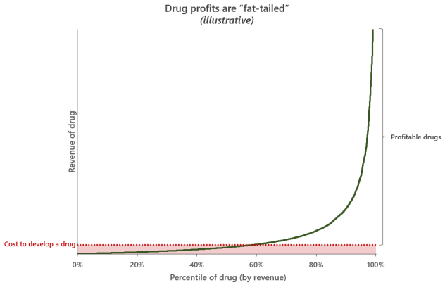
As illustrated by the graph above, the cost of developing a drug is relatively bounded, but the potential return on investment in any one drug is extreme with the top selling drugs recouping many multiples of their initial development expenses. In this sense, developing a drug is conceptually like buying a “lottery ticket”. It’s obvious that to maximize the potential opportunity, as many drugs should be developed as possible. The strategy of maximizing exposure to upside potential with call-option-like bets (fixed price, unlimited potential return) is one that Nassim Nicholas Taleb talks about a lot in Antifragile. But is this a better strategy than focused bets on expensive late-stage drugs? I believe a look at base rates and some simple modelling can be informative here.
Portfolio strategy takeaways
In the “Appendix” of this post I walk through the methodology and results of the simulations I ran to explore these questions, but if you don’t want to read all that my takeaways for portfolio strategy from that analysis are below:
- The distribution of pharmaceutical product revenues appears to fit a “fat-tailed” distribution well (specifically, a lognormal distribution), which means that a small number of hugely successful drugs will drive most of the return on investment for the entire pharmaceutical market
- If the amount invested in a drug to bring it to market is greater than the probability of launch * median lifetime drug revenue at each phase it is unlikely to generate more revenue than it cost to develop
- It’s not inherently better to focus on maximizing probability of success (an “exploit” strategy) or number of drugs in a portfolio (an “explore” strategy). What is important is to maximize the expected value in terms of number of expected launches as cheaply as possible, which can be calculated simply by summing up the probability of launch for each drug in a portfolio.
- There is a fairly large “scale premium” that means portfolios with large expected number of launches return more on a per product basis than smaller portfolios; the more launches, the more chances of a mega-blockbuster that will recoup the costs of multiple poorly performing launches.
Of course, there are many other qualitative factors that are important in the commercial success of a drug (e.g. sales force expenditure, efficacy/safety, unmet need, competitors, etc.) that were not discussed in this post. But I think there is value in considering the implications of an aggregated statistical view before layering on these additional considerations.
Appendix
Part 1 – Estimating parameters for portfolio simulation:
After some tinkering and attempts to fit several different distributions to sales data, I found the distribution of annual pharmaceutical sales revenue (in millions of USD) appears to be relatively well approximated by a lognormal distribution with a σ value of 1.5 (the standard deviation of the natural log of the distribution), which is a value of σ at which the top 10% of the distribution accounts for ~60% of the total value, and a μ value of 5 (the mean of the natural log of the distribution).
Assuming that there are roughly 1,800 drugs on the market (which is in line with the total number of new molecular entities approved by the FDA7), drawing that many samples from a lognormal distribution with the previously outlined σ and μ parameters and calculating the sum of those values should provide a rough estimate of the total value of the pharmaceutical market – which ends up being ~$770bn, close to EvaluatePharma’s estimate8 of $764bn in 2019. These parameters can also generate the kinds of top-heavy distributions observed in reality, as seen in a representative example of the top 10 values from a sample of 1,800 vs. the top 10 drugs by 2019 revenue in the graphs below:
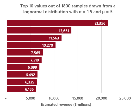
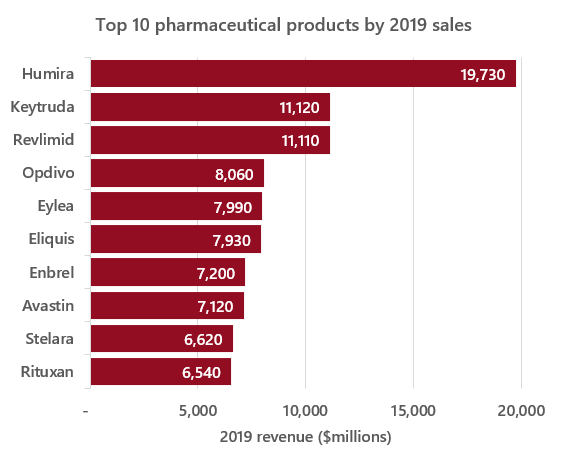
Source: https://www.fiercepharma.com/special-report/top-20-drugs-by-global-sales-2019
Next, estimating the distribution of cumulative lifetime product revenue. If we assume that cumulative lifetime revenue is roughly 10x annual revenue (A few years less than the ~13 year average time from launch to loss of exclusivity9), we can then use \(log(12 * e^5) = ~7.3\) as our new μ value. This new μ value seems to produce values at the high end of the distribution in line with real values (see comparative example below).
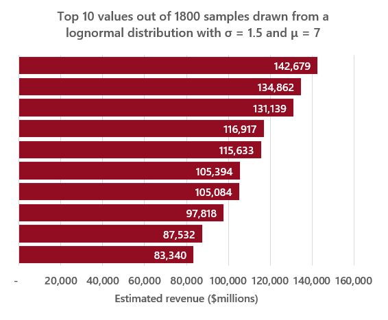
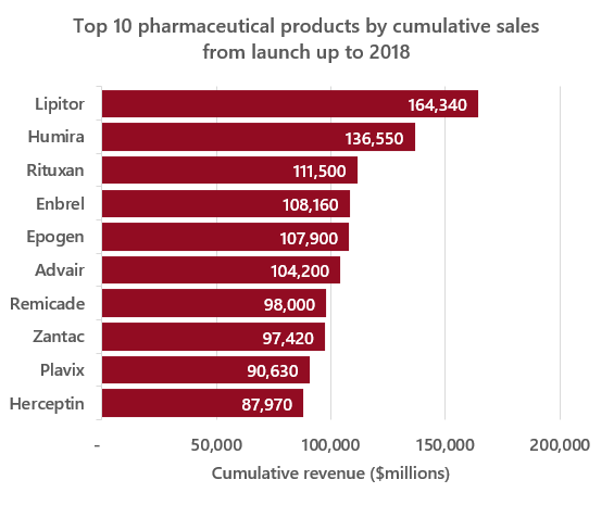
Source: https://www.statista.com/statistics/1089322/top-drugs-by-lifetime-sales-globally/
These parameters imply an expected value of cumulative lifetime sales for a drug of ~$4.6 billion, by the lognormal distribution expected value formula:
\[e^{(μ + σ^2/2)}\]which is broadly in line with published values1011. Obviously these are imperfect estimates, but I am reasonably comfortable using them in the context of this post.
Part 2 – Estimating the expected values of drugs by development stage:
Returning to our original scenario, and assuming that returns from pharmaceuticals do follow a lognormal distribution, we can estimate the expected value of a drug with the following formula:
\[-c(1 - P(launch)) + P(launch) * (e^{(μ + σ^2/2)} - c)\]Where P(launch) is the probability of reaching the market and c is the cost associated with each drug (to acquire, license, develop, etc.). This is essentially the expected value of the binomial probability function combined with the expected value of a lognormal distribution. Assuming 0 value for drugs that fail to launch.
So, if we use our assumptions outlined above (σ = 1.5, μ = 7.3) and set c to 0 then plug the values into the expected value formula, we get the following expected values for a single random drug in each stage of development:
| Probability of launch | Expected value of drug in stage | |
|---|---|---|
| Start of phase 1 | 7% | $319m |
| Start of phase 2 | 15% | $684m |
| Start of phase 3 | 62% | $2,827m |
| Launched | 100% | $4,560m |
Estimated values of P(launch) by phase from a recent article in Nature Reviews Drug Discovery12
Which implies that if you’re constructing an arbitrarily large portfolio of pipeline drugs, this is roughly the amount that should be invested in each drug of each phase to break even on the eventual returns (i.e. what value c should be in the formula above). The caveats being this simple analysis doesn’t account for inflation, discount rate, etc. nor does it account for possibility of spreading the investment over multiple phases (i.e. the cost to develop a drug to launch is not all paid upfront).
However, it is important to note that the median of a lognormal distribution is given by \(e^μ\), which is ~$1,480m with our parameters, which indicates that we expect the majority of launches to make substantially less than the expected value, as most of the value lies in the fat tail of the distribution.
Part 3 – Simulating portfolios:
Finally, I returned to the original question of whether it’s better to invest in many cheap, early stage drugs (an “explore” strategy) or fewer, but late stage drugs (an “exploit” strategy). To start with I simulated portfolios that varied by the number of drugs and probability of launch of the underlying drugs to understand the trade-offs between these two factors, assuming a cost per drug equal to the expected value calculated above.
To simulate portfolios, I first calculated the number of successful launches in each portfolio of size n using the values in the table above, then drew a sample at random from a lognormal distribution (with parameters σ = 1.5, μ = 7.3) for the number of successes given by n – n(failures). The value of the portfolio was calculated as the sum of the values of all successes minus the cost per drug times n (see python code at the bottom of this post for details).
Results of simulating 10,000 early stage portfolios, each paying the expected value of $319m per drug:
- With 1 phase 1 drug ~94% of portfolios lose money (most portfolios contain no launched drugs)
- With 5 phase 1 drugs ~84% of portfolios lose money
- With 10 phase 1 drugs ~79% of portfolios lose money
- With 100 phase 1 drugs ~66% of portfolios lose money
- With 1,000 phase 1 drugs ~59% of portfolios lose money
Results of simulating 10,000 late stage portfolios, each paying the expected value of $2,827m per drug:
- With 1 phase 3 drug ~80% of portfolios lose money
- With 5 phase 3 drugs ~70% of portfolios lose money
- With 10 phase 3 drugs ~65% of portfolios lose money
- With 100 phase 3 drugs ~60% of portfolios lose money
- With 1,000 phase 3 drugs ~55% of portfolios lose money
Clearly, the expected return of a portfolio is sensitive to the number of drugs in that portfolio, as having more drugs leads to more chances that the portfolio will include one of those rare products with massive revenues. In fact, it doesn’t matter whether you try to maximize number of drugs or probability of launch, as portfolios with equivalent values of \(number of drugs * P(launch)\) have equivalent outcomes (this is in line with the expected value of a binomial distribution). To illustrate this, I simulated the outcomes for the three portfolio constructions below, all with an number of drugs * P(launch) value of 3.1:
- 44 phase 1 drugs, each paying the expected value of $319m per drug
- 21 phase 2 drugs, each paying the expected value of $684m per drug
- 5 phase 3 drugs, each paying the expected value of $2,827m per drug
For each of these portfolio variants, approximately 30% of simulated portfolios make money. The implication is that a pharmaceutical company should try to maximize the value of number of drugs * P(launch) for their pipeline as cheaply as possible. Additionally, it is notable that paying the calculated expected value per drug will mean most portfolios will lose money, regardless of construction.
Finally, I wanted to estimate a cost per drug where >=50% of portfolios would make money. For a single drug this is relatively straightforward, you solve for c in the below formula and pay that amount (i.e. for a single drug with 100% P(launch) you should pay the median of the lognormal distribution).
\[-c(1 - P(launch)) + P(launch) * (e^{μ} - c) = 0\]However, the lognormal distribution is not stable13, which means that the distributions of the sums of sets of n > 1 samples drawn from the distribution will be different than the distribution of single samples (which is clear from the simulation results above). In our case, this property confers a “scale premium” to larger portfolios vs. smaller ones.
To estimate the magnitude of this scale premium I simulated 50 sets of portfolios (2,000 simulated portfolios per set) ranging from 1 to 50 drugs each with 100% P(launch) and plotted the median portfolio value divided by the number of drugs in each portfolio (graph below, the line of best fit is a logistic function, x axis is the number of drugs per portfolio, y axis is the median portfolio value divided by number of drugs per portfolio).
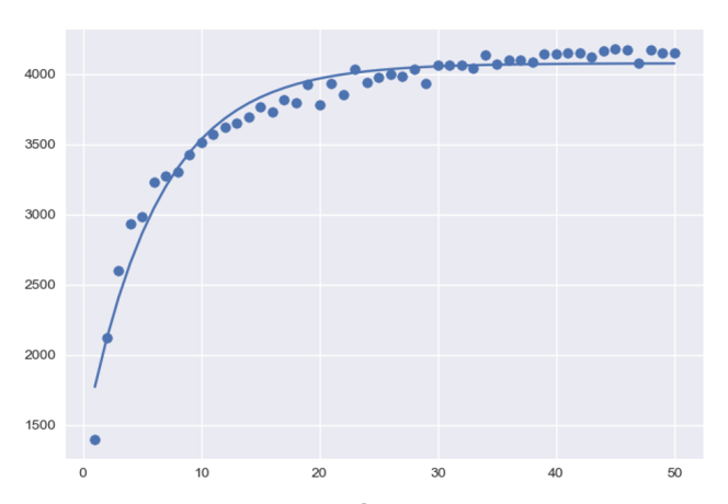
This means that (with our parameters) between 0-10 drugs the returns to scale on expected value are large, but the scale premium flattens after that. The implication is that companies benefit from larger portfolios and should in theory have a greater willingness to pay to develop new drugs if their portfolios are already large (in this example a company with 20 expected launches in their portfolio should be willing to pay ~2x as much to develop a new drug as a company with only 2 expected launches).
You can find the code I used for the simulations on github here
-
https://media.nature.com/original/magazine-assets/d41573-019-00074-z/d41573-019-00074-z.pdf ↩
-
https://pubmed.ncbi.nlm.nih.gov/11151306/ ↩
-
https://pubmed.ncbi.nlm.nih.gov/12457422/ ↩
-
https://pubmed.ncbi.nlm.nih.gov/30644967/ ↩
-
https://pubmed.ncbi.nlm.nih.gov/25646104/ ↩
-
https://www.forbes.com/sites/davidshaywitz/2017/07/26/the-startling-history-behind-mercks-new-cancer-blockbuster ↩
-
https://pubmed.ncbi.nlm.nih.gov/24680947/ ↩
-
https://info.evaluate.com/rs/607-YGS-364/images/EvaluatePharma_World_Preview_2019.pdf ↩
-
https://www.statnews.com/wp-content/uploads/2017/01/Lifetime_Trends_in_Biopharmaceutical_Innovation.pdf ↩
-
https://pubmed.ncbi.nlm.nih.gov/30644967/ ↩
-
https://pubmed.ncbi.nlm.nih.gov/25646104/ ↩
-
https://media.nature.com/original/magazine-assets/d41573-019-00074-z/d41573-019-00074-z.pdf ↩
-
https://en.wikipedia.org/wiki/Stable_distribution ↩