Developing a deeper understanding of diagnosis rates
If you’ve ever seen (or built) a patient-based prevalence model to forecast revenue for a pharmaceutical product it’s likely that “proportion of patients diagnosed” was one of the inputs used in that model to estimate the number of potential patients likely to take that particular drug. However, it’s been my experience that good information on the true prevalent diagnosed proportion of a particular condition is rarely available, and in lieu of better data some token assumption in the range of 80-95% is used. Sometimes you can make use of published cross-sectional prospective screening studies to find a solid estimate of the true proportion of diagnosed patients, but more often than not you’re forced to make an educated guess.
I don’t want to use unjustified and arbitrary assumptions in forecasts if I can avoid it, so I tried to explore the topic and learn a bit more about it, guided by three main questions:
- If I don’t have access to the true value of the proportion of diagnosed patients, what other variables can I use to estimate that value and how important are they?
- Average or median time to diagnosis is much easier to come by in the literature than “proportion of patients diagnosed”. What impact does a faster or slower diagnosis have on the proportion of patients diagnosed?
- What do I need to believe to find a particular value of “proportion of patients diagnosed” in a model plausible?
My approach was to break the problem down in a few variables that seem influential for determining the “proportion of patients diagnosed”, then sketch a simple model and use values for those variables from the literature to identify likely boundaries on plausible values for the “proportion of patients diagnosed”. I walk through my approach over the next few sections, but if you want to skip to my takeaways they’re at the end of the post.
A few definitions to start
- “Patients” are people with a specific medical condition, whether or not they have a confirmed diagnosis
- For brevity I will refer to the “proportion of patients with a confirmed diagnosis” as \(p(Dx+)\), which is equivalent to the probability that a randomly chosen patient has a confirmed diagnosis at the time of selection. \(p(Dx+)\) is calculated by dividing the number of living patients with a confirmed diagnosis by the total number of living patients, whether or not they have a confirmed diagnosis
- \(p(Dx-)\), the “proportion of patients without a confirmed diagnosis”, is equal to \(1 - p(Dx+)\)
- Diagnostic delay is the “time interval between the onset of symptoms and confirmed diagnosis of a disease”1
A simple model of the path to diagnosis
If you take a cross-sectional sample of a population with a given chronic disease, patients will either have a confirmed diagnosis at that specific time, or they won’t. But a simple value of \(p(Dx-)\) captures two very different groups of people:
- Patients who are in the process of getting a diagnosis, and will get it some time in the future if they survive long enough to complete the diagnostic process
- Patients who will never get a confirmed diagnosis because they are not seeking one and/or not being screened (perhaps they have an asymptomatic condition and have no particular reason to visit a doctor)
The question I then had was “Which is a bigger contributor to low rates of diagnosis, a slow diagnostic pathway or non-care seeking behaviour?
I’ve sketched out a toy model to help outline the contributors to a particular value of \(p(Dx+)\) below, assuming that patients can be in one of four distinct states:
- Undiagnosed, seeking treatment (\(Seeking\ Dx\))
- Undiagnosed, not seeking treatment (\(Not\ seeking\ Dx\))
- Diagnosed (\(Dx+\))
- Dead
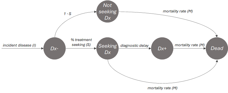
In this toy model the proportion diagnosed is dependent on 3 factors: the treatment seeking rate (\(S\)), the diagnostic delay and the mortality rate (\(M\)). We can treat the \(Seeking\ Dx\) group as a sort of queue; if patients are able to remain in that group for \(t\) time steps without succumbing they will enter the \(Dx+\) group. So the toy model reveals a natural opposition between the mortality rate and rate of diagnosis, and at a high-level how \(p(Dx+)\) depends on diagnostic delay.
The longer the diagnostic delay, the less chance that someone is diagnosed before they die (whether or not it’s directly related to the disease) and the more people that are in the diagnostic pathway relative to the diagnosed population.
An equation for p(Dx+)
If you make a few (likely untrue, albeit useful) simplifying assumptions you can make use of a fairly simple equation to calculate \(p(Dx+)\) at steady state, based on the structure of the toy model above:
- First, I assume that time to diagnosis is symmetrically distributed (like a normal distribution). With this assumption I can represent the diagnosis rate as the average or median time to diagnosis (\(t\)), because in a symmetric distribution a patient is just as likely to be diagnosed earlier than average as they are to be diagnosed later
- Second I assume that all patients have the same mortality rate, regardless of whether or not they have a diagnosis
Thereby, the equation is as follows:
\[p(Dx+) = (1 - M)^t * S\]What this equation is effectively saying is that at each time step \(t\), \(1 - M\) percent of patients in the undiagnosed population will die. By the time you have waited for \(t\) time steps, the number of patients that remain i.e. \((1 - M)^t\) will be the diagnosed population (since everyone dies at the same rate in our model). Then, you remove people who aren’t seeking treatment by multiplying by \(S\) to get to a final estimate of the proportion diagnosed.
If you set \(S\) to 1 and plot \(p(Dx+) = (1 - M)^t\) you get a graph like the one below, which visualizes the opposition between the mortality rate and rate of diagnosis I mentioned earlier.
From this graph we can make the following observations:
- \(p(Dx+)\) tends to fall off very quickly to zero with increasing values of \(t\) and/or \(M\)
- However, if either \(t\) or \(M\) are very low (near 0), \(p(Dx+)\) is relatively insensitive to high values of the other variable
Reducing the value of \(S\) simply scales the height of the graph down proportionally.
Base rates of mortality (M), average time to diagnosis (t) and treatment seeking (S)
Next I wanted to find some real values of \(M\), \(t\) and \(S\) from the literature and plug them into my basic model, in the hope of finding some informative relationships.
Base rates of diagnostic delay (t)
To get some data on what a “typical” time to diagnosis is, I collected a set of papers that chronicle median or mean diagnostic delay for a variety of conditions. All in all from my quick search of PubMed I found 94 data points which I plotted below:

In my (non-comprehensive) sample, the mean is 41 months, the median is 25 and the interquartile range is 6 to 50; this suggests that most conditions take about 1 to 4 years to diagnose. I also grouped conditions into therapy areas, which showed that oncology tended to be much faster to diagnose than other conditions, generally taking a few months, which makes sense given the urgency and relatively hard diagnostic criteria.
Notably, there are a few outliers that skew the upper end of the distribution, mainly rare conditions such as hereditary haemorrhagic telangiectasia (25.7 years mean diagnostic delay2), erythropoietic protoporphyria (13 years mean diagnostic delay3) and late onset Pompe disease (12 years mean diagnostic delay4).
Base rates of mortality (M) in the general population, and a comparison of diagnostic delay (t) to mortality rates for specific conditions
The overall crude mortality rate in the general population is ~1% per year per World Bank data5, but as you can see in the table from the WHO6 below it varies drastically by age group. Below age 55 the annual risk of death is very small (<1% per year), but it increases drastically thereafter to ~18% per year in over 85s.
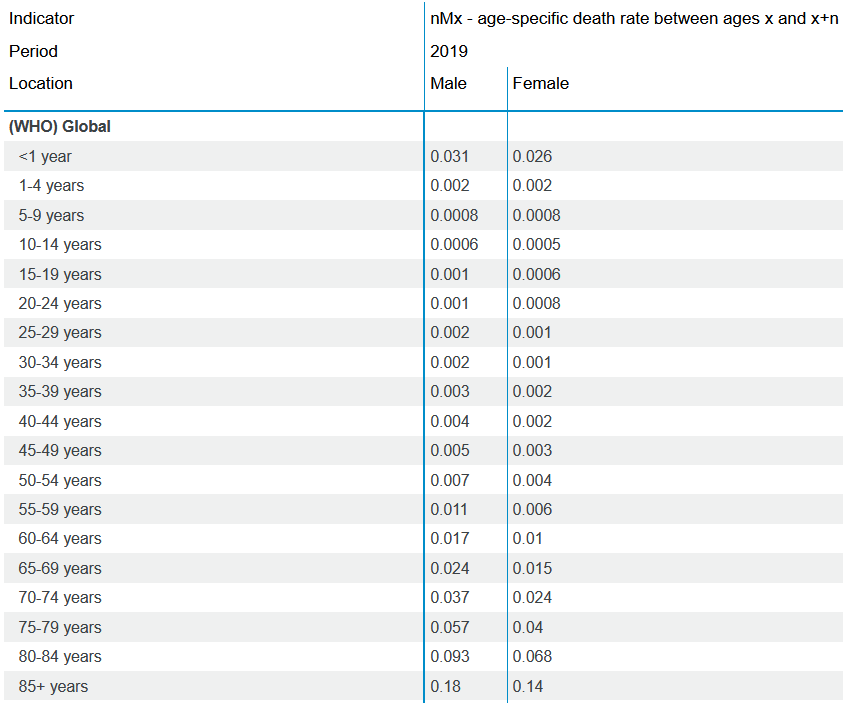
So we might expect most chronic conditions without a strong impact on life expectancy to have crude mortality rates of ~1%, in-line with the general population. However, obviously many conditions increase mortality rates substantially compared to the general population.
I suspected that high mortality conditions would tend to have low diagnostic delays (due to the urgency to treat), and vice versa. So I collected and plotted some published data on mortality rates (post-diagnosis) for a variety of conditions below (interesting examples annotated). I took a crude approach to selecting and synthesizing the mortality rate data (i.e. just including whatever I could easily find on PubMed and roughly approximating annual mortality rates from whatever they reported), but I think the data is suggestive of a relationship between the two variables.
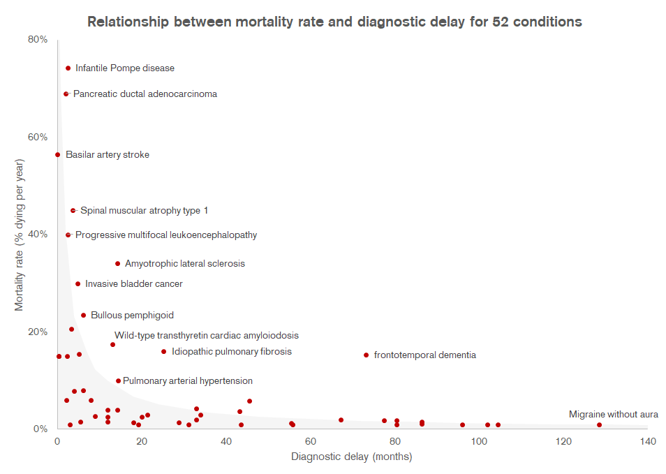
Grey area shows the threshold at which \(p(Dx+)\) is predicted to be 90% based on the formula \(p(Dx+) = (1 - M)^t * S\), assuming that \(S\) = 1. The faint gray dotted line is set at 1%, which is the approximate general mortality rate in the overall population
If you plug the datapoints I’ve plotted above into the formula for \(p(Dx+)\) above, assuming that all patients seek treatment (i.e. \(S\) = 1), we’d estimate that the vast majority of conditions in the sample would have a \(p(Dx+)\) value over 90% (shown by the grey area on the graph). Most conditions in my (admittedly small) sample seem to get diagnosed quite quickly if their mortality is high. Vice versa, if the diagnostic delay is long (e.g. migraine, narcolepsy) mortality is also likely low enough that it doesn’t matter if it takes years for a diagnosis to be confirmed, almost everyone will survive long enough to get one. A condition with a mortality rate of ~1% would need to have a diagnostic delay of over 10 years to dip below 90% \(p(Dx+)\), assuming everyone seeks care.
Some of the conditions above the 90% envelope such as frontotemporal dementia probably do have low \(p(Dx+)\) rates as a result of diagnostic delays, likely stemming from complex differential diagnostic procedures and/or lack of urgency to confirm a specific diagnosis due to a lack of treatment options.
So what does this mean? Well, my hypothesis is that low real-world values of \(p(Dx+)\) are probably not in most cases a result of long diagnosis delay or high mortality rates. I think it’s more likely that when we do observe low values of \(p(Dx+)\) in reality it’s primarily a result of low rates of treatment seeking.
Base rates of treatment seeking (S)
\(S\) should reflect the proportion of people who never seek treatment, because a tendency to delay treatment seeking is baked into the average diagnostic delay. It’s hard to find information on this in the literature, but what I could find was fairly consistent in suggesting that 25% to 30% of people avoid seeking general medical care (e.g. for influenza-like illness), even if they recognize a need for it78910. Obviously the more subjectively severe a condition, the more likely someone is to seek care. Conversely, people with asymptomatic conditions may only seek a confirmatory diagnosis if they have particular risk factors or a family history. A generally non-serious condition such as acne can be expected to have lower rates of treatment seeking, e.g. ~17%11. In practice this value will probably be difficult to get hard data on, but 70-75% seems like a reasonable base case value for \(S\) in many instances.
Takeaways
- Most non-lethal, chronic conditions should have high values of \(p(Dx+)\). I think a solid “naive” estimate for \(p(Dx+)\) for chronic conditions is ~90% without taking \(S\) into account, and ~65% if you do. I guess I agree with the generic 80-95% assumptions I’ve seen in practice after all!
- The most significant contributor to low rates of \(p(Dx+)\) is probably in most cases a low rate of treatment seeking behaviour (very rare diseases aside), implying that most initiatives to focus on improving \(p(Dx+)\) should focus on increasing the propensity of patients to seek care
- Initiatives that speed up time to diagnosis only make a big impact on \(p(Dx+)\) if mortality rates are high, although they can help improve patient quality of life by speeding up time to treatment initiation
- Treatment seeking influences diagnosis rates, and shouldn’t be “double counted” in forecasts
Appendix:
The data from the literature I used to make my graphs above are summarized in this Excel file
Adapting the model for acute conditions
The formula \(p(Dx+) = (1 - M)^t * S\) works more naturally for chronic conditions than acute, but a simple alternative for acute conditions could be something like the below:
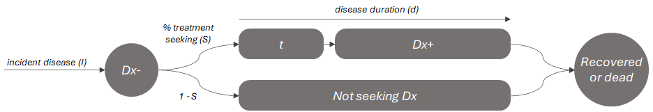
Where the value of \(p(Dx+)\) is approximated by the ratio of time spent with a confirmed diagnosis (\(Dx+\) or \(d - t\)) to the total duration of the disease (\(d\)), multiplied by the treatment seeking rate (\(S\)).
For example, influenza lasts around 8 days once it becomes symptomatic12. If we assume that 70% of symptomatic people would seek care at all (per references above), and it takes ~2 days to get a diagnosis on average after the onset of symptoms we would estimate \(p(Dx+)\) to be the following:
\[p(Dx+) = (\frac{d - t}{d}) * S\] \[p(Dx+) = (\frac{6}{8}) * 0.7\] \[p(Dx+) = 0.525\]Implying a rough estimate that ~53% of active symptomatic influenza cases have a confirmed diagnosis at any given time, which seems plausible. If we add another term to account for asymptomatic infections the total value of \(p(Dx+)\) could be an additional 50-80% lower13
-
https://en.wikipedia.org/wiki/Diagnostic_delay ↩
-
https://pubmed.ncbi.nlm.nih.gov/22676497/ ↩
-
https://pubmed.ncbi.nlm.nih.gov/30041937/ ↩
-
https://pubmed.ncbi.nlm.nih.gov/31497486/ ↩
-
https://databank.worldbank.org/source/gender-statistics/Series/SP.DYN.CDRT.IN ↩
-
https://www.who.int/data/gho/data/indicators/indicator-details/GHO/gho-ghe-life-tables-by-country ↩
-
https://pubmed.ncbi.nlm.nih.gov/29249189/ ↩
-
https://pubmed.ncbi.nlm.nih.gov/24556894/ ↩
-
https://pubmed.ncbi.nlm.nih.gov/32220247/ ↩
-
https://pubmed.ncbi.nlm.nih.gov/31565121/ ↩
-
https://pubmed.ncbi.nlm.nih.gov/22888857/ ↩
-
https://pubmed.ncbi.nlm.nih.gov/27486731/ ↩
-
https://pubmed.ncbi.nlm.nih.gov/26133025/ ↩