Ergodicity and biotech, or why expected value is a mirage

“Don’t cross a river if it is four feet deep on average” - Nassim Nicholas Taleb

Setting the scene: the expected value of clinical development

Expected value calculations are a typical way to evaluate whether or not investment in a particular clinical development program is likely to be financially worthwhile. To calculate expected value, one lays out all the potential outcomes of a clinical development program, such as in the flow chart in figure 1 below, estimates the net profit/loss for each potential path, and sums up the values of each of the paths weighted by their probability. The timing of revenues and costs can then be used to discount the expected value by conversion to a net present value (NPV). These articles provide a nice overview of the commonplace “risk-adjusted NPV” valuation practice in biotech.

Figure 1: A flowchart showing a simplified and high-level clinical development process. Starting on the left, there are five potential paths through the process to get to the two possible end states: launch or failure

Historically, the industry-wide return on investment for biopharma research and development has been sufficiently positive to support a thriving sector; ~$800bn is spent on branded (innovator) medicines annually worldwide¹. Supporting this assertion, I (roughly) estimate that the lifetime expected value of a typical clinical development program is ~$209 million (without net present value discounting), implying that investing in drug development is on average a good bet (see calculations in appendix 1 at the end of the post).

Despite the positive expected value, it is well known that drug development programs are both expensive and unlikely to succeed. Historical probability of success rates in the industry indicate that ~92% of programs fail at some point in clinical development², and with full clinical development programs costing hundreds of millions of dollars the price of failure is high. While estimates vary, costs per approved drug are likely $1 billion or higher if you account for the costs of failed trials³. Worryingly, in recent years influential analyses⁴⁵ have suggested that the return on investment for biopharmaceutical research and development is declining and may turn negative in the near future as the best opportunities are exhausted.

At face value, it may seem hard to reconcile the positive expected value of drug development with the fact that the vast majority of clinical development programs lose tens if not hundreds of millions of dollars for no return. In order to maintain a positive return on investment, the rewards of successful innovation must be massive to offset the high cost and risk of clinical development. The dichotomy of outcomes - costly failure or riches - results in outliers driving the vast majority of the returns in biopharma⁶⁷. The median clinical biopharmaceutical company is a perennial money-loser, but the success of the Genentech’s, Amgen’s and Gilead’s of the world more than makes up for the losses of companies that never bring a product to market. Survivorship bias can give us an overly rosy picture of the chance of success, and a positive industry-wide expected value can mask the underlying risks for individual programs.

Ergodicity and the problems with expected value

Ergodicity is a concept that originated in thermodynamics, with relatively recent popularization in economics and finance circles through the work of Ole Peters⁸ and Nassim Nicholas Taleb⁹. In essence, a system is ergodic if averaging the state of a single member of the system over a long period of time (the time average) gives you an equivalent result to taking the average of the states of all the members of a system at a specific time (the ensemble average). This definition implies that an ergodic system does not have inescapable attractor states which trap members of the system and prevent them from visiting all the possible states of the system over a long enough time period, as shown in figure 2 below.

Expected value calculations implicitly assume that you are operating in an ergodic system, where the expected value represents the average outcome over an infinite amount of trials or an infinite number of members of the system. While it’s common to use an expected value based approach to evaluate the attractiveness of a single development program in isolation, it really only becomes meaningful when applied to many different programs over long periods of time. Furthermore, the real world is mostly non-ergodic; there are plenty of absorbing attractor states (e.g. death) and you are constrained by your resources and the results of your previous actions. To quote Ole Peters:⁸

“An expectation value of a non-ergodic observable physically corresponds to pooling and sharing among many entities. That may reflect what happens in a specially designed large collective, but it doesn’t reflect the situation of an individual decision-maker… We all live through time and suffer the physical consequences of the actions of our younger selves.”

The world that biopharmaceutical companies operate in is a non-ergodic one, where a failed trial program for a cash-strapped biotech is likely to land it squarely within the terminal attractor states of bankruptcy and dissolution. The history of one particular company is unlikely to provide much information about the fates of all companies; failure is likely, and failed companies cease to exist without ever capturing the ostensibly positive expected value of investing in clinical development.

A biopharmaceutical company using expected value to make decisions about investment opportunities has to contend with three key problems with the metric:

Outcomes in biotech are binary, companies either make a fortune or spend a huge amount of money with nothing to show for it. As such, the expected value for a single development program is an illusion that quantifies the non-existent middle ground between extreme outcomes
Expected value is insensitive to context; two bets with the same expected value can have wildly divergent risk profiles (see appendix 2 for a simple example)
Pursuing decisions on the basis on maximizing expected value does not necessarily provide the best path to long-term success, as it tells you little about which decisions minimize the risk of ruin

In an ergodic world of infinite time, capital and opportunities for investment these problems can be safely ignored, as the law of large numbers smooths away any volatility. However, ignoring these problems in the real (non-ergodic) world may prove ruinous.

Simulating expected value in a non-ergodic system

To visualize the problems with expected value I built a simple simulation app included directly in this post below (if you’re not seeing it it may take ~60 seconds to load). The app is pre-populated with probability of success and cost benchmarks from the literature, and uses these values to simulate the outcomes for 100 model biotechs as they attempt up to 50 successive clinical development programs, implementing the algorithm outlined by the flowchart in figure 1.

I set the simulated biotechs to each start with $500m by default. Each clinical trial a simulated biotech attempts costs a certain amount of money, such that with the default settings each biotech can initially afford just over one full development program (from phase 1 up to and including regulatory submission). If these biotechs are lucky enough to succeed in all the development phases and launch a drug they immediately receive a lump sum of cash pulled from a lognormal distribution (I explain the rationale for this distribution and the default parameters in this other post.

For as long as they have more than $0, each biotech will continually attempt a full development program paying the costs specified in the cost boxes. If a biotech’s money drops below $0 they are considered bankrupt (indicated by a red trace on the large graph), and they can no longer pursue additional clinical development programs. The possibility of bankruptcy is the attractor state that introduces non-ergodic behaviour into the simulation.

The simulation below is interactive, and if you like you can re-run it after plugging new values into the grey boxes below the graphs to see how these affect the overall outcomes and likelihood of bankruptcy. Refresh the page to restore the default values.

A note on limitations: I wanted a straightforward simulation, so I made the following simplifications:

Simulated biotechs can only work on one program at a time
All the lifetime revenue of a launched drug is captured instantly at the time of launch
There are no non-R&D costs
Simulated biotechs cannot raise additional money outside of what they start with or receive in revenues from launches

I’ve plotted three averages in blue lines on the main graph: the theoretical expected value (if no biotechs could go bankrupt), the actual average and the average of only the non-bankrupt biotechs. Survivorship bias is visualized in the difference between the expected value and the dark blue line above. If ruin was not a possible outcome, then we would see all three curves be equal as biotechs that were unlucky early on would be able to catch-up later (you can test this by inputting 1 for all the probabilities of success).

Clearly this is an overly simplistic simulation that doesn’t account for non-R&D costs, nor does it spread costs and revenues over time as in the real world. Nevertheless, there are two conclusions that are readily apparent when running the simulation with the default parameters:

Roughly 85% of biotechs go bust, typically quite rapidly
Once the biotechs get past a certain level of capital, they will tend to survive long-term

The results of the simulation imply the presence of absorbing attractor states to both the upside and downside, and a clear bifurcation in the natural histories of biotechs. The critical takeaway from the simulation is that the real average value captured by the simulated biotechs over successive programs is almost always lower than the theoretical expected value under the default conditions, because of the potential for ruin.

How much cash is enough?

In the simulation, long-term survival is achieved once a biotech has enough of a capital buffer to survive “unlucky” drawdowns due to failure of clinical development programs. Because the expected value is positive with the default parameters, the simulated companies will make positive returns on investment and accrue capital over time as long as they can afford to repeatedly invest in clinical development programs.

In the real world, big pharma cash hoards and venture capital portfolios can be large enough to benefit from a positive expected value, but small biotechs cannot reliably capture the expected value in any meaningful sense. Large amounts of cash give you the luxury of being able to ignore the system’s non-ergodicity. But how much cash is enough to provide a sufficiently sizeable buffer such that almost all biotechs are protected from bad luck and hence are able to survive long-term?

If you plot the influence of starting money in the simulation above on the proportion of bankrupt biotechs you get a nice fit to an exponential function, as shown in figure 3 below. (The best fit function is approximately $e^{-0.00021x}$, where $x$ is the starting cash, in case you’re curious). As starting capital increases companies are exponentially more likely to survive long-term, up to a point at which almost all companies survive (~$10bn or so with the default simulation parameters). The implication of this is that the amount of cash a company has to spend on R&D is a reasonably good predictor of how likely a biotech is to survive indefinitely.

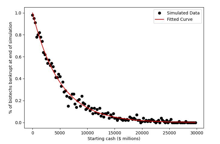
Figure 3: The influence of starting cash on the proportion of non-bankrupt biotechs at the end of the simulation with default parameters. As starting cash increases, more and more biotechs survive to the end of the simulation

This all being said, clinical development programs are long. A full development program takes ~10 years (~2 years for phase 1, ~3.5 years each for a phase 2 or 3 and ~1 year for regulatory approval)²¹⁰. With typical burn rates on the range of $30-50m per annum per program a biotech on the road to ruin with a few hundred million in cash may lumber on as one of the “walking dead” for upwards of a decade before finally succumbing.

Tying it all together

In summary, expected value (or NPV, if you prefer) is commonly used to make development decisions as it is presumed to quantify the real current value of investing in a clinical development program. However, expected value is a flawed measure in the real non-ergodic world with problems whether it is applied to evaluate single programs or many programs over time.

When used to evaluate the value of a single program in isolation the expected value tells you little about what to expect from the outcome of the program as the variance and range of possible outcomes are abstracted away into a single value. As most outcomes in biotech are binary the number is only meaningful across an (infinitely) large number of trials. Unfortunately, applying expected value across many development programs in the hope that the variance in outcomes will eventually average out is not necessarily a safe approach either, as over time the risk of ruin means that real captured value is likely lower than the theoretical cumulative expected value.

Expected value should be interpreted differently depending on your current state (i.e. amount of money), and the likelihood of a ruinous outcome. Large well-capitalized companies can make use of expected value as it was intended, because they have the money to run many experiments across a portfolio (although they may be constrained by the number of good investment opportunities). Large cash reserves (or high cash flow) is an effective moat in a capital intensive, high-risk industry like biopharmaceuticals because you can benefit from the positive expected value accrued over many development programs while maintaining enough of a buffer to survive failures, and your new cash-poor competitors are fragile and likely to go out of business. This dynamic is why we saw the attractors pulling companies towards enduring success or failure emerge out of the simulation.

As biotechs plan their investments in development programs it may be prudent for them to also think about their exposure to non-ergodicity and ruinous outcomes. If cash is limited, simply selecting the option with the highest expected value may expose them to unacceptable risk (see appendix 3 for a simple example). The more harmful the downside of a decision is, the less relevant expected value is and the more important it is to focus on the probabilities of specific outcomes instead. It’s not particularly meaningful to work out the expected value of a game of Russian roulette, for example.

One good way to incorporate a more nuanced approach into decision making is through simulation of the potential discrete outcomes. I’d argue that all decision makers would benefit from an understanding of what each distinct possible future of a development program entails for their company’s long-term survival. Instead of maximizing expected value, does it make sense to optimize for the probability of ruin-avoidance instead?

Additionally, small biotechs can consider specific strategies to make them more robust over the longer term. Asset consolidation, as we’ve seen with companies like BridgeBio and Centessa could be a good mechanism of ruin avoidance as a single successful development programs can often repay the costs of many failures.

Appendix 1: Estimating the expected value of a typical clinical development program using industry benchmarks

Expected value is defined as the following equation, where $x_i$ is the value of a particular outcome $i$, $p_i$ is the probability of that outcome occurring and $k$ is the number of potential different outcomes.

\[E(X) = \sum_{i=1}^{k} p_i * x_i\]

In order to calculate the expected value for a typical clinical development program we will need some assumptions for the probability of success and cost (or profit) for each phase of development, as well as the potential revenue for a launched product:

For probability of success I’ll use values from a 2021 BIO report², shown in figure 4 below.

Figure 4: Phase transition success rates from phase 1 for all diseases, all modalities as of 2020. Source: BIO, Biomedtracker, Pharmapremia

For costs I will use the average values from the supplementary data of the paper “Estimated Research and Development Investment Needed to Bring a New Medicine to Market, 2009-2018”³, shown in the table below:

I will assume that regulatory submission costs are $2.9 million, per 2021 FDA PDUFA fee guidance¹¹.

In anther post I estimated the expected value of a drug launch to be ~$4.6 billion (in terms of cumulative lifetime revenue), so I’ll use that value here too.

With reference to figure 1, there are five potential outcomes in our simple model of a clinical development program:

Failing in phase 1
Succeeding in phase 1 then failing in phase 2
Succeeding in phase 1 and 2, then failing in phase 3
Succeeding in phase 1, 2 and 3, then being rejected by regulators
Succeeding in all phases, being approved by regulators, then launching the drug

Using the assumptions outlined above, I have calculated below the value of each of the scenarios:

Failing in phase 1

Scenario likelihood = $48\%$

\[(P1\ cost * (1 - P1\ PoS))\] \[(-\$52.9m * (1 - 52\%)) = -\$25.4m\]

Succeeding in phase 1 then failing in phase 2

Scenario likelihood = $37\%$

\[((P1\ cost + P2\ cost) * (P1\ PoS*(1 - P2\ PoS)))\] \[((-\$52.9m + -\$100.8m) * (52\%*(1 - 28.9\%))) = -\$56.8m\]

Succeeding in phase 1 and 2, then failing in phase 3

Scenario likelihood = $6.3\%$

\[((P1\ cost + P2\ cost + P3\ cost) * (P1\ PoS*P2\ PoS*(1- P3\ PoS))\] \[((-\$52.9m + -\$100.8m + -\$291.6m) * (52\%*28.9\%*(1-57.8\%))) = -\$28.2m\]

Succeeding in phase 1, 2 and 3, then being rejected by regulators

Scenario likelihood = $0.8\%$

\[((P1\ cost + P2\ cost + P3\ cost + Reg\ cost) * (P1\ PoS*P2\ PoS*P3\ PoS*(1- Reg\ PoS))\] \[((-\$52.9m + -\$100.8m + -\$291.6m + -\$2.9m) * (52\%*28.9\%*57.8\%*(1 - 90.6\%)) = -\$3.7m\]

Succeeding in all phases, being approved by regulators, then launching the drug

Scenario likelihood = $7.9\%$

\[((P1\ cost + P2\ cost + P3\ cost + Reg\ cost + Expected\ Revenue) * (P1\ PoS*P2\ PoS*P3\ PoS*Reg\ PoS)\] \[((-\$52.9m + -\$100.8m + -\$291.6m + -\$2.9m + \$4,600m) * (52\%*8.9\%*57.8\%*90.6\%) = \$323.6m\]

Overall expected value

\[-\$25.4m + -\$56.8m + -\$28.2m + -\$3.7m + \$323.6m = \$209.4m\]

Implying that investing in a typical clinical development program is expected to be a good bet, netting ~$209m per program on average.

Appendix 2: Expected value is insensitive to context

Scenarios with the same expected value can nevertheless have a distinct character. Take the following example: almost everyone would be willing to risk $1 for a 10% chance to win $100, this is very favourable in expected value terms (+$9).

\[(90\% * -\$1) + (10\% * (\$100 - \$1)) = \$9\]

However, would you be willing to bet $1,000,000 for a 10% chance to win $10,000,090? This has the same expected value as the above bet, so in expected value terms it should be equally as appealing as the first bet.

\[(90\% * -\$1,000,000) + (10\% * (\$10,000,090 - \$1,000,000)) = \$9\]

I suspect that the vast majority of people would be unwilling to take the second bet as they would be risking a 90% chance of losing a ruinous amount of money. While most people can absorb the loss of $1 without financial ruin, very few can absorb the loss of $1,000,000. It is only the rich few who would be able to benefit from this type of bet, and hence the individual context of the bet-taker has a huge impact on the wager’s attractiveness. This second bet is analogous to what biopharmaceutical companies do, i.e. risk significant amounts of capital for a small chance of making a fortune.

Appendix 3: A positive expected value can mask underlying risks

I want to use a very simple example to illustrate how a positive expected value could lead decision makers astray. Let’s imagine a biotech was selecting between two products to invest in, we’ll call them product X and product Y. Let’s also imagine the biotech has a budget of $455m to spend on R&D.

Product X has the following costs and probabilities of success for each phase of development:

Product X	Phase 1	Phase 2	Phase 3	Regulatory submission
Cost	$50m	$100m	$300m	$5m
Probability of success	100%	100%	10%	100%

If product X succeeds the company expects $5,000m in cumulative revenues, but running the program would cost the company’s entire R&D budget. The expected value of developing product X is therefore:

\[(90\% * -\$450m) + (10\% * (\$5,000m - \$455m)) = \$45m\]

On the other hand, product Y’s costs and probabilities of success are as follows:

Product Y	Phase 1	Phase 2	Phase 3	Regulatory submission
Cost	$35m	$60m	$200m	$5m
Probability of success	30%	100%	100%	100%

If product Y succeeds the company expects only $500m in cumulative revenues. The expected value of developing product Y is therefore:

\[(70\% * -\$35m) + (30\% * (\$500m - \$300m)) = \$36m\]

If the biotech decides to invest in product X they will most likely spend all their money for a 10% chance of success. If they go for product Y they are 3x more likely to launch a product but the upside is 10x smaller. However, if they do fail they will fail at an early point where they have not spent much, and will have enough cash left over to try again with another program. I posit that most of the time product Y is the better choice, even with a lower expected value and upside potential.

This is not a particularly realistic example, but it shows some of the dangers with pursuing an expected value maximization strategy and the value of failing early in avoiding exposure to the risk of ruin.

https://www.iqvia.com/insights/the-iqvia-institute/reports/global-medicine-spending-and-usage-trends-outlook-to-2025 ↩
https://go.bio.org/rs/490-EHZ-999/images/ClinicalDevelopmentSuccessRates2011_2020.pdf ↩ ↩² ↩³
https://pubmed.ncbi.nlm.nih.gov/32125404/ ↩ ↩²
https://endpts.com/pharmas-broken-business-model-an-industry-on-the-brink-of-terminal-decline/ ↩
https://www2.deloitte.com/us/en/pages/life-sciences-and-health-care/articles/measuring-return-from-pharmaceutical-innovation.html ↩
https://pubmed.ncbi.nlm.nih.gov/29220034/ ↩
https://twitter.com/biotechyoda/status/1487021639082467330 ↩
https://www.nature.com/articles/s41567-019-0732-0 ↩ ↩²
Skin in the Game: Hidden Asymmetries in Daily Life ↩
https://www.nature.com/articles/nrd.2017.21 ↩
https://www.fda.gov/industry/fda-user-fee-programs/prescription-drug-user-fee-amendments ↩